Tail Integral Formula for Expected Value

Try this original problem before opening the solution. Then compare the method with SOA Exam P sample question 50.

Original practice · fully worked

Original variant: capped emergency-power demand

A remote clinic’s emergency energy demand D has survival function P(D>x)=(3/x)² for x at least 3 kilowatt-hours. A battery can supply at most 12 kilowatt-hours. Find the expected energy actually supplied.

C
3.750 kWh
B
4.500 kWh
A
5.250 kWh
D
5.625 kWh
E
6.000 kWh

Show the answer and worked solution

Answer and calculation

Integrating the survival probability up to the battery ceiling gives 3 plus 9 times the integral of x⁻² from 3 to 12, or 5.25 kWh.

Setup

Let the supplied energy be the smaller of D and 12. The survival probability is one below the minimum demand 3 and equals 9 divided by x squared thereafter.

S_D(x)=1\ (0\le x<3),\qquad S_D(x)=9x^{-2}\ (x\ge3)

Model

For a nonnegative demand, the expected amount delivered up to capacity 12 is the integral of its survival function from zero to 12.

E[\min(D,12)]=\int_0^{12}S_D(x)\,dx

Compute

The interval from 0 to 3 contributes 3. Integrating the inverse-square survival function from 3 to 12 contributes 2.25, for a total of 5.25.

E[\min(D,12)]=3+9\int_3^{12}x^{-2}\,dx=3+9\left(\frac13-\frac1{12}\right)=5.25

Answer

Therefore the battery supplies 5.250 kWh on average, corresponding to choice A.

\boxed{5.250\ \text{kWh}\quad\text{(A)}}

Technique orientation

What tail integral formula and expected value questions are testing

For a nonnegative random variable, expected value is the area under its survival curve: E[X] = ∫₀∞ P(X > t) dt. The identity is useful when the survival function is simpler than the density, and it extends directly to deductibles and limits once the payment variable—not merely the ground-up loss—is defined.

The November 2026 SOA Exam P syllabus assigns 44–50% of the exam to univariate random variables and requires candidates to explain and calculate expected values, including moments, and insurance payments. The 46 verified solutions below connect that official scope to tail integrals, direct sums or integrals, linearity, and conditioning.

Recognition audit

Signals that this is the right method

A nonnegative variable is described through P(X > t), a survival function, or a CDF whose complement is easy to integrate.
The question asks for a mean loss, average payment, premium, expected count, or long-run cost.
A deductible or limit turns the requested payment into a transformed variable whose tail has clear thresholds.
Several groups or stages suggest conditioning first and then averaging conditional expectations.

Before calculation

A disciplined first pass

Name the requested quantity, mark its units or time point, and identify the assumption that permits the formula. Only then insert the numerical inputs. This separates model errors from arithmetic errors and makes the answer-choice comparison auditable.

Formula core

Tail Integral Formula and Expected Value formulas to know

These identities are starting points, not substitutes for checking support, timing, rate periods, or independence assumptions.

LOTUS

E[g(X)]=\sum_x g(x)p_X(x)\quad\text{or}\quad E[g(X)]=\int g(x)f_X(x)\,dx

Use the sum or integral over the support of X; a transformed density is not required.

Linearity

E\!\left[\sum_j a_jX_j+c\right]=\sum_j a_jE[X_j]+c

Linearity does not require independence.

Tail integral

X\ge0\quad\Longrightarrow\quad E[X]=\int_0^\infty P(X>x)\,dx

This is the area under the survival function. The nonnegative condition is essential for this one-integral form.

Discrete tail sum

X\in\{0,1,2,\ldots\}\quad\Longrightarrow\quad E[X]=\sum_{k=1}^{\infty}P(X\ge k)

Write each integer value as the number of positive thresholds it crosses.

Deductible and limit

Y=\min((X-d)_+,u)\quad\Longrightarrow\quad E[Y]=\int_d^{d+u}P(X>x)\,dx

This is payment per loss. Payment per payment would additionally condition on X > d.

Three failure modes to catch

Using the single nonnegative tail integral for a variable that can be negative without separating its positive and negative parts.
Integrating the CDF F(x) instead of the survival function 1 − F(x), or continuing beyond finite support.
Computing payment per loss when the question asks for payment per payment, which requires conditioning on a positive payment.

Tail integral proof

Why expected value is the integral of the survival function

For every realized nonnegative value x, the indicator 1{x > t} equals one from t = 0 up to x. Integrating that indicator recovers x itself. Tonelli's theorem then permits the order of expectation and integration to be exchanged because the integrand is nonnegative.

Derivation

Layer the random variable by threshold

Start with the pointwise layer identity X = ∫₀∞ 1{X > t} dt for X ≥ 0.
Take expectations on both sides. Nonnegativity permits the expectation and integral to be exchanged even when the mean is infinite.
For each threshold t, E[1{X > t}] is exactly P(X > t), the survival function Sₓ(t).
Therefore E[X] = ∫₀∞ Sₓ(t) dt. A finite upper support replaces infinity with that endpoint.

Worked example

Exponential lifetime

If X has mean 500, its survival function is exp(−t/500). The tail integral should return the same 500-unit mean.

E[X]=\int_0^\infty e^{-t/500}\,dt=500

Check: The result matches the reciprocal-rate check and has the same time unit as X.

Worked example

Payment after a deductible and limit

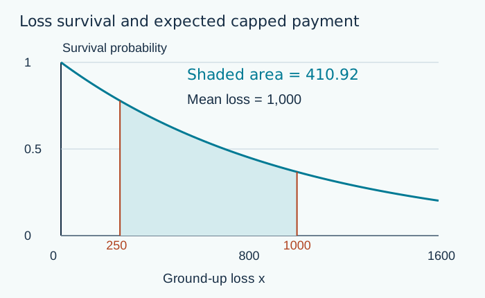
Let X be exponential with mean 1,000. For Y = min((X − 250)₊, 750), integrate the loss survival only from 250 through 1,000.

E[Y]=\int_{250}^{1000}e^{-x/1000}\,dx=1000(e^{-0.25}-e^{-1})\approx410.92

Check: The expected payment is positive and below the 750 payment limit.

Compare the conditioning

Survival curves: loss, payment and positive payment

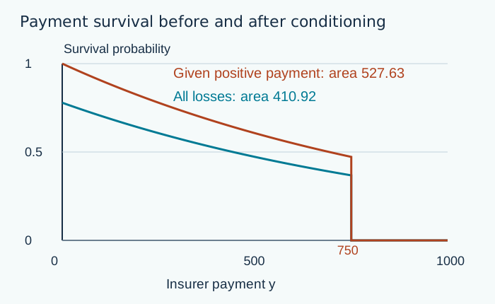
The deductible-and-limit example above uses the area from loss 250 to loss 1,000. The shaded curve and the payment comparison below show why the mean changes when zero payments are excluded.

Exponential loss survival curve with shaded area from loss 250 to 1000. Its shaded area is the expected capped payment, 410.92. — Loss X is exponential with mean 1,000. Payment Y = min((X − 250)₊, 750). The shaded area is E[Y] = 410.92.

Capped payment survival and survival conditional on positive payment. Both drop to zero at the 750 payment limit. The conditional curve starts at one and has a larger area. — The conditional curve starts at one and has area E[Y | Y > 0] = 527.63. The unconditional curve starts at 0.778801 and includes the zero-payment losses.

Same loss model; different payment definition or conditioning
Quantity	Deductible	Payment limit	P(positive payment)	Mean per loss	Mean per positive payment
Ground-up loss X	0	None	1.000000	1,000.00	1,000.00
Deductible only (X − d)₊	250	None	0.778801	778.80	1,000.00
Deductible and payment limit	250	750	0.778801	410.92	527.63

At the 750 payment limit the survival function is zero: the payment cannot exceed the cap. The positive left limit before that drop is the probability mass at the cap. At payment zero, the unconditional survival starts at P(X > 250), while conditioning on a positive payment starts at one. Dividing the unconditional mean by P(X > 250) recovers the conditional mean.

Use the one-integral formula only for a nonnegative variable. A signed variable needs its positive and negative tails separated; linearity of expectation itself does not require independence. Continue with the exponential distribution problems and worked formula examples.

Download the four-page diagrams and condition checks (free PDF).

Original ActuaryProof diagrams and calculations, October 1, 2026. Personal study and unchanged redistribution with attribution are permitted. This independent study aid is not an official SOA handout or material permitted in the exam.

Verified practice ledger

Exam P tail integral formula and expected value problems and solutions

The list is grouped by current official syllabus area. Every link opens a step-labeled solution, verification artifact, distractor analysis, and one fully worked original variant.

General Probability

6 verified references

SOA Exam P Sample Question #74Binomial DistributionVerified
SOA Exam P Sample Question #81Conditional ProbabilityVerified
SOA Exam P Sample Question #98Expected ValueVerified
SOA Exam P Sample Question #360Discrete Random VariablesVerified
SOA Exam P Sample Question #405Expected ValueVerified
SOA Exam P Sample Question #415Inclusion-ExclusionVerified

Univariate Random Variables

32 verified references

Multivariate Random Variables

8 verified references

Continue the study loop

Keep every worked reference in one searchable manual

The complete Exam P manual includes all active sample-reference solutions, their wrong-choice analysis, and one independently written worked variant per reference. The free formula sheet is the compact companion for recall between practice sessions.

The page and all 46 linked browser solutions are free. The $19 Probability Formula & Distribution Cards is a 44-page PDF with 72 formula cards. The $49 Probability Proof Manual is 3,108 pages with 718 worked solutions plus 718 original variants.

Inspect 72 formula cardsView contents and sample pagesGet the free formula sheet

Related drills

Other Exam P technique collections

Switch techniques when you can identify the current method before writing a formula and can explain each wrong-choice mechanism.

103 verified problems

Conditional Probability

Conditioning, total probability, and Bayes calculations organized around the denominator that defines the updated sample space.

83 verified problems

Exponential Distribution

Waiting-time probabilities, parameter conversions, memorylessness, moments, and insurance-payment applications.

72 verified problems

Poisson Distribution

Count probabilities, rate scaling, aggregation, thinning, and links between Poisson counts and waiting times.

62 verified problems

Normal Distribution

Standardization, inverse percentiles, linear combinations, normal approximations, and tail control.

57 verified problems

Variance

Second moments, transformations, sums, covariance terms, and conditional variance decompositions.

55 verified problems

Independence

Event independence, factorization, independent trials, and the consequences independence does—and does not—justify.

50 verified problems

Uniform Distribution

Continuous and discrete uniform models, interval geometry, transformations, order statistics, and moments.

Sources and accountability

Primary sources and correction path

SOA: November 2026 Exam P syllabusDefines the current exam format, the 44–50% univariate-random-variable weight, expected-value outcomes, and insurance-payment scope.
Official Exam P sample questionsThe numbered references linked above originate in this official question set.
Official Exam P sample solutionsUsed to verify answer choices; ActuaryProof writes its own explanations and variants.

ActuaryProof publishes the independent explanations on this page. Official exam facts on this page come from the sources above; schedules, study ledgers, and checking protocols are ActuaryProof editorial tools unless stated otherwise. Read about the publisher or report a suspected error.

Primary sources last checked: September 26, 2026.